Solar Highways Monitoring
End report
01-01-2019 – 30-06-2020
End report for Action C2 Monitoring of the impact of the project actions, as described in the Grant Agreement LIFE13ENV/NL/000971 Solar panels as integrated constructive elements in highway noise barriers (June 2014).
Net energy produced from 1-1-2019 to 30-06-2020: 325.5 MWh
Authors: Simona Villa & Minne de Jong
Date: 13-08-2020
1. Introduction
1.1. The Solar Highways Bifacial Solar Noise Barrier
The Solar Highways bifacial noise barrier was monitored for energy performance from commissioning of the system until 30 June 2020. The specifications for the energy performance system were part of the procurement documentation. The equipment was installed and initially tested by the contractor, Heijmans. The inverter system is supplied by SolarEdge. Every solar laminate is connected to two SolarEdge power optimizers, enabling monitoring on module level through the SolarEdge monitoring portal. For accurate measurements, AC power meters were installed measuring the total net production (and consumption). Eight AC power meters were installed: one for every of the six ‘experiment sections’ and two for the main parts of the system.
1.2. Solar noise barrier specifications
The solar noise barrier consists of 268 solar laminates, each containing 194 solar cells. Each laminate is 3 meters wide and 2 meters high. Two laminates are framed together and made into a cassette. Two cassettes are placed on top of each other between poles to form a section.
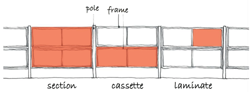
Figure 1. Elements of the solar noise barrier.
In total, the solar noise barrier is composed of 67 sections, which can be subdivided in 2 production areas and 6 test/experimental areas. A schematic of the of the subdivision is shown in Figure 2. In particular, we have:
- Production area 1: made of 37 elements;
- Production area 2: made of 18 elements;
- Test area 1, 2, 3, 4, 5, 6: made of 2 elements each.
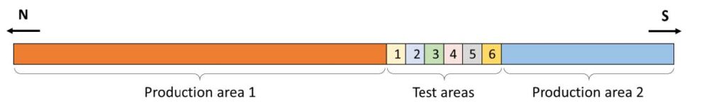
Figure 2. Schematic showing the different areas of the solar noise barrier.
1.3. Flash data
Flash data was provided by the contractor. In the specifications of the contractor, the rated power of the laminate was set at 887 Wp (+/- 10%) and a bifaciality factor of 65%. The flash data by the manufacturer shows rated powers on the front side (the ‘sunny’ side) ranging from 836 to 967 Wp, with an average of 926 Wp. Therefore the total front side rated power is 4.5% higher than rated power in the contract. The back side rated powers range from 580 to 715 Wp with an average of 655 Wp, such that the average bifaciality factor is 70.8%. The rated powers of front and back side, as well as the bifaciality factor, of each area are summarized in Table 1.
| Prod. 1 | Prod. 2 | Test 1 | Test 2 | Test 3 | Test 4 | Test 5 | Test 6 | Total SH | |
| Front side [kW] | 137.412 | 66.580 | 7.336 | 7.307 | 7.322 | 7.441 | 7.482 | 7.450 | 248.331 |
| Back side [kW] | 97.111 | 47.182 | 5.239 | 5.177 | 5.202 | 5.314 | 5.249 | 5.356 | 175.830 |
| Total [kW] | 234.523 | 113.762 | 12.575 | 12.484 | 12.523 | 12.755 | 12.732 | 12.806 | 424.161 |
| Bifaciality [%] | 70.7 | 70.9 | 71.4 | 70.8 | 71.0 | 71.4 | 70.2 | 71.9 | 70.8 |
Table 1. Rated power and bifaciality factor of each production and test area.
1.4 Module mapping
The module manufacturer provided a ‘mapping’ that shows the position of each module in the solar noise barrier, such that the total rated power for each section can be determined. It also shows the serial numbers of the power optimizers, such that the performance of the optimizers in the SolarEdge monitoring platform can be linked to the location in the solar noise barrier.
2. Monitoring setup
2.1. Monitoring equipment
The type and accuracy of the different measurement sensors was defined in the procurement documents. The following equipment was installed:
- Eight Janitza UMG 604-UMG power meters were installed. One for every ‘experiment section’ and two for the main parts of the system.
- Three Kipp and Zonen SMP3 pyranometers were installed: one on the east side and one on the west side of the solar noise barrier, both in the same orientation as the barrier. The third one was installed horizontally on top of the noise barrier.
- SolarEdge provides module level power monitoring on their online portal: monitoring.solaredge.com
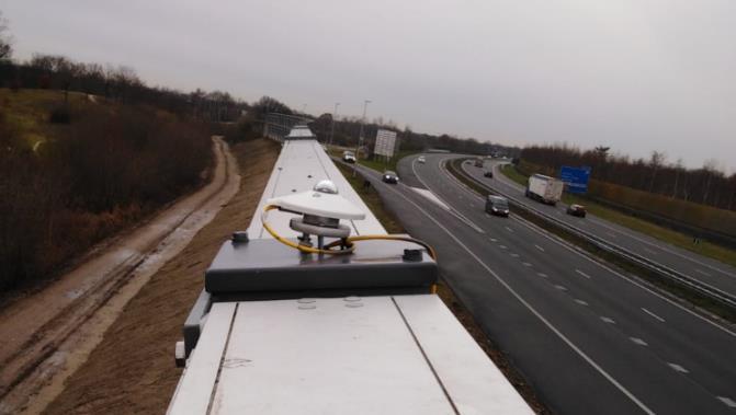
Figure 3. Horizontally mounted pyranometer.
2.2. Data flows
Five-minutely data from the power meters and the pyranometers is recorded. At the end of every day, data for that day is transferred to a TNO server, where it is further processed. The SolarEdge data can be viewed semi-realtime, as well as historical data. After some initial hiccups, a stable data flow since mid-December 2018 is recorded. At TNO this is further processed for analysis.
2.3. Monitoring tools
The system performance can be viewed through two different systems: the SolarEdge monitoring system and the Grafana monitoring tool, based on the AC power readings and irradiance measurements. The following tools are available:
- ΤΝΟ monitoring system: link (requires login)
- Net electricity generation
- Irradiation
- SolarEdge
3. Monitoring results
The monitoring results will be presented at first considering a reference clear-sky day, so that typical irradiance and output profiles can be observed and analyzed. Then, the performance results of the solar noise barrier will be evaluated for the complete 18-month period, from 1st January 2019 to 30th June 2020.
3.1. Typical sunny day
As reference sunny day we considered the 27th of February 2019. Figure 4 shows the horizontal and in-plane irradiations on both East and West side of the vertical PV modules, as well as the sum of these two (highlighted in red). Differently from a south-oriented PV system, the vertical bifacial solar noise barrier receives two clearly distinguished peaks of solar radiation, during morning on the East side and during afternoon on the West side. Around noon, the irradiation is parallel to the barrier and almost no direct light is received by the modules. Throughout the whole day, the diffuse light component gives its contribution to the total irradiance. The solar noise barrier is tilted 10° towards the East side with respect to the vertical, hence we would expect the West irradiance peak to be higher than the Eastern one. However, as can be seen in the figure 4, the opposite result is measured. The reason for this is due to the fact that the highways is not perfectly aligned to the North/South (N/S) orientation, but it deviates of a few degrees in the direction N-E/S-W. The impact of this effect on the irradiance profile is also dependent on the Sun’s position and elevation, therefore the shape of the irradiance doubled-peak profile will change throughout the year.
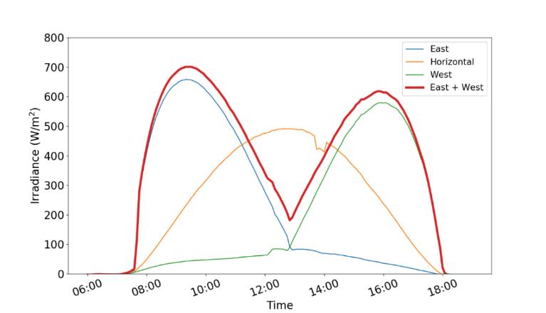
Figure 4. Comparison between in-plane irradiances on East side, West side, sum of both sides and global horizontal.
Figure 5 shows the output power of one of the experimental zones together with the effective irradiance, i.e. the irradiation on both sides of the modules keeping into account the bifaciality factor. The effective irradiance can be calculated as:
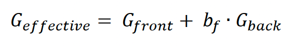
where G front is the West irradiance, G back is the East irradiance and b f=0.71 is the bifaciality factor used in the calculations. In this way we can compare the profile of the actual energy produced with the theoretical input solar energy. The normalized irradiance now shows a higher peak during the afternoon, when the direct sunlight hits the front part of the barrier. As shown in the graph, this profile is matched by the power production. However, it can be observed that around midday the power output profile presents a low plateau.
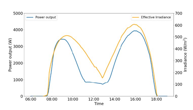
Figure 5. Power output and effective irradiance.
To understand the reason behind this we can compare the output profile with the performance ratio of the module, calculated according to:
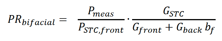
Using this formula, the measured electrical output is scaled to the STC performance of the best performing side of the cell (front side). The used PR definition, therefore, already takes into account the bifaciality factor, which is the ratio of the front and back STC efficiency of the modules.
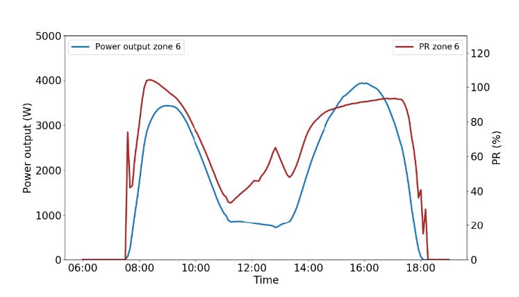
Figure 6. Output power compared to PR (test area 6).
From Figure 6, we can clearly see that the performance of the PV modules decreases starting from the morning hours up to early afternoon. These dips in PR are caused by the so-called construction shading: shading coming from the vertical and horizontal supporting structures of the solar noise barrier elements. This effect can also be observed when plotting the power output versus the bifacial irradiance (Figure 7). Every point that deviates from a linear dependence proves the presence of shade. It can be observed that the strongest shading effect takes place during the morning hours.
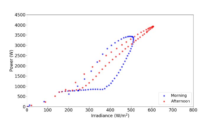
Figure 7. Power versus irradiance measurements to show non-linearity due to shading.
Figure 8 and Figure 9 show the PR ratio of the two production areas and the six test areas, respectively. The average daily PR for this reference sunny day ranges from 76 to 82% for the different solar noise barrier zones.
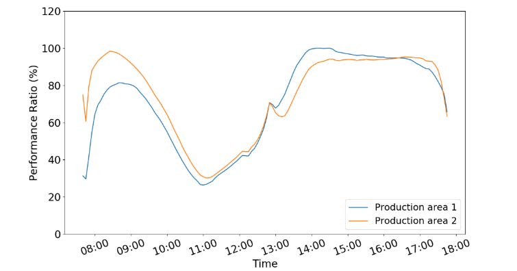
Figure 8. PR profile of the two production areas
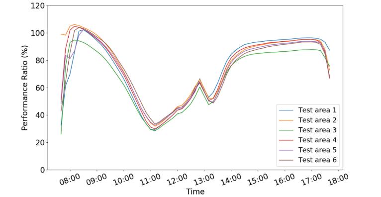
Figure 9. PR profile of the six test areas
It is interesting to compare the power profiles of single sunny days for each month of the year, as shown in Figure 10. It is possible to observe how the double-peak profile “evolves” during the year, scaling up and increasing its afternoon peak when approaching summer months.
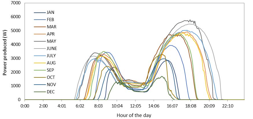
Figure 10. Power profile of a sunny day for each month of the year 2019.
3.2. Overall performance and energy output
In Figure 11, the daily net energy output of the whole solar noise barrier has been plotted for the complete 18-month period, from the start of January 2019 to the end of June 2020. Daily and seasonal fluctuations are clearly visible in the figure, such as the exceptionally high PV production in the spring 2020 due to the very high irradiation recorded. On 05/05/2020 the solar noise barrier set its highest record, producing 1.65 MWh of clean electricity on a single day.
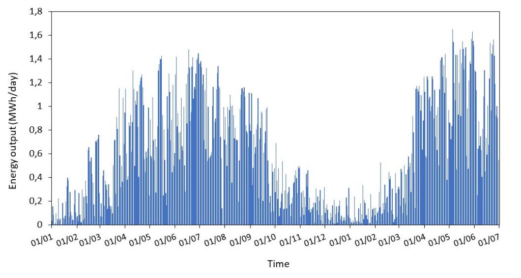
Figure 11. Daily net energy output of the whole solar noise barrier.
Figure 12 shows the daily PR of the whole system¹. Generally, the days characterized by very low PR values, e.g. below 60%, do not indicate a bad performance of the PV noise barrier, but only that parts of the system were shut down due to maintenance works. Maintenance works include, for example, replacement of connectors, replacement of damaged glass and general investigation, and those took place mostly in January/February 2019, May/June 2019 and from around December 2019 to February 2020.
¹ PR calculations have been performed up to the 5th of June 2020 because of the interruption of the TNO monitoring system (including power data from the power meters and irradiance data from the pyranometers). Power data for the month of June were retrieved from the SolarEdge portal.
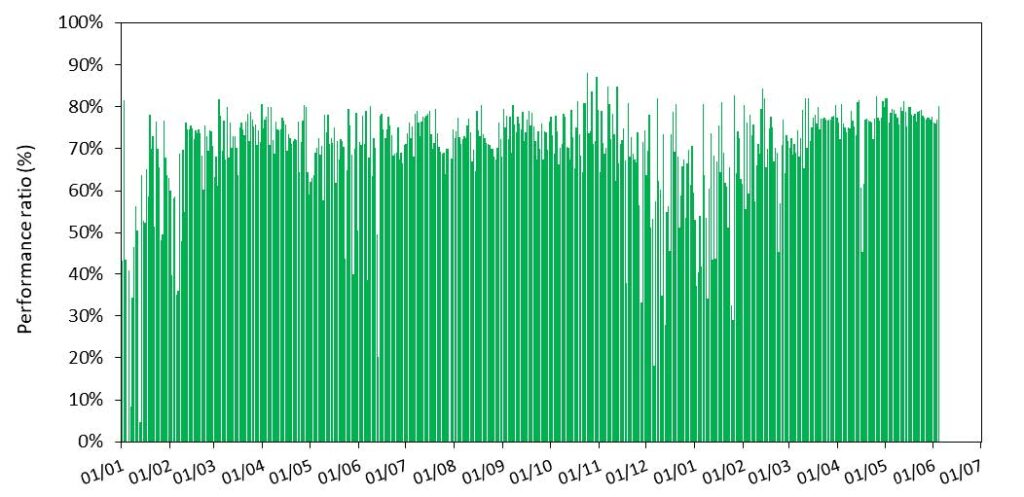
Figure 12. Daily overall performance ratio of the whole solar noise barrier.
Figure 13 and Table 2 show the monthly breakdown of the total energy output of the solar noise barrier, differentiating between the different areas.
The net yearly energy yield for 2019 was 202.84 MWh/year, corresponding to an AC specific yield of 816.8 kWh/kWp. The total output of the 18-month period amounts to 325,5 MWh.
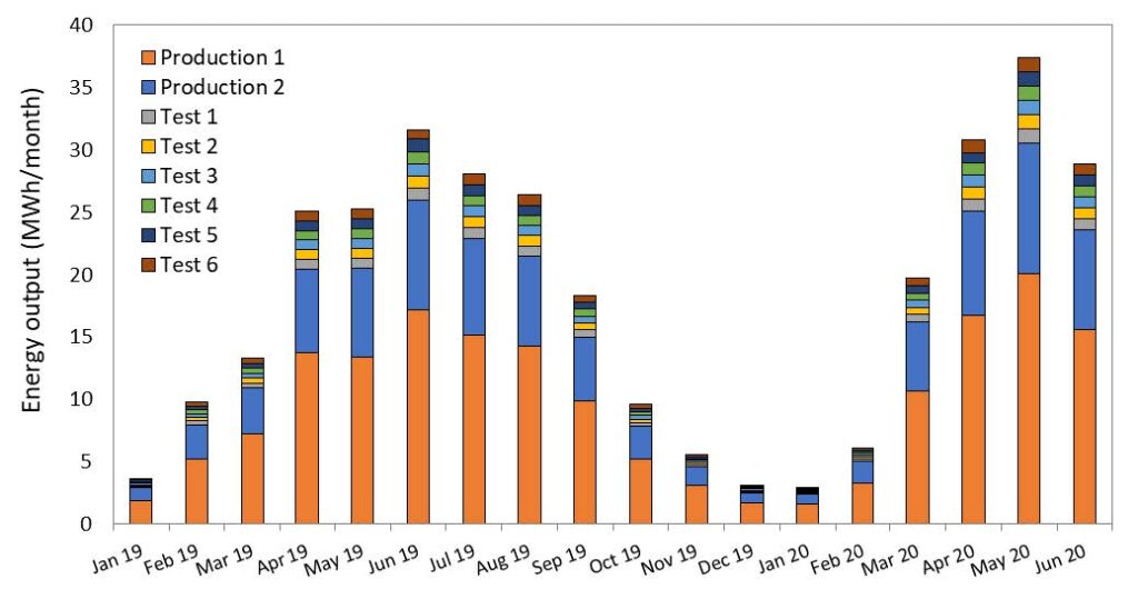
Figure 13. Breakdown of solar noise barrier energy production for every month.
| Prod 1 | Prod 2 | Test 1 | Test 2 | Test 3 | Test 4 | Test 5 | Test 6 | TOTAL | |
| Jan 2019 | 1,901 | 1,005 | 0,124 | 0,110 | 0,122 | 0,123 | 0,124 | 0,125 | 3,634 |
| Feb 2019 | 5,234 | 2,695 | 0,307 | 0,280 | 0,305 | 0,303 | 0,305 | 0,312 | 9,741 |
| Mar 2019 | 7,214 | 3,666 | 0,403 | 0,380 | 0,400 | 0,398 | 0,397 | 0,404 | 13,264 |
| Apr 2019 | 13,687 | 6,791 | 0,777 | 0,768 | 0,780 | 0,771 | 0,759 | 0,781 | 25,113 |
| May 2019 | 13,347 | 7,213 | 0,793 | 0,783 | 0,796 | 0,782 | 0,778 | 0,789 | 25,281 |
| Jun 2019 | 17,124 | 8,860 | 0,980 | 0,973 | 0,979 | 0,971 | 0,983 | 0,758 | 31,628 |
| Jul 2019 | 15,099 | 7,832 | 0,865 | 0,860 | 0,862 | 0,860 | 0,867 | 0,829 | 28,074 |
| Aug 2019 | 14,212 | 7,315 | 0,815 | 0,808 | 0,810 | 0,806 | 0,806 | 0,842 | 26,414 |
| Sep 2019 | 9,886 | 5,089 | 0,561 | 0,555 | 0,553 | 0,550 | 0,556 | 0,572 | 18,322 |
| Oct 2019 | 5,183 | 2,653 | 0,286 | 0,284 | 0,284 | 0,282 | 0,285 | 0,296 | 9,552 |
| Nov 2019 | 3,070 | 1,525 | 0,169 | 0,168 | 0,150 | 0,168 | 0,168 | 0,175 | 5,592 |
| Dec 2019 | 1,704 | 0,811 | 0,095 | 0,096 | 0,096 | 0,096 | 0,095 | 0,099 | 3,091 |
| Jan 2020 | 1,608 | 0,764 | 0,087 | 0,088 | 0,086 | 0,087 | 0,086 | 0,090 | 2,897 |
| Feb 2020 | 3,316 | 1,677 | 0,186 | 0,187 | 0,188 | 0,187 | 0,187 | 0,194 | 6,121 |
| Mar 2020 | 10,679 | 5,461 | 0,606 | 0,599 | 0,603 | 0,598 | 0,583 | 0,622 | 19,752 |
| Apr 2020 | 16,725 | 8,380 | 0,993 | 0,984 | 0,975 | 0,902 | 0,858 | 0,965 | 30,782 |
| May 2020 | 20,101 | 10,425 | 1,149 | 1,152 | 1,153 | 1,145 | 1,139 | 1,166 | 37,431 |
| Jun 2020 | 15,554 | 8,053 | 0,875 | 0,880 | 0,881 | 0,876 | 0,876 | 0,880 | 28,886 |
Table 2. Monthly energy yield of all production and test areas for the complete period.
The monthly performance ratio of the production areas and test areas are respectively shown in Figure 14 and Figure 15, and summarized in Table 3.
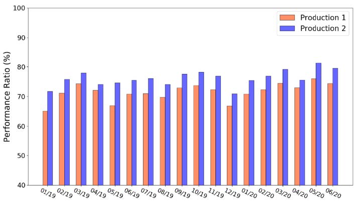
Figure 14. Monthly PR of the two production areas.
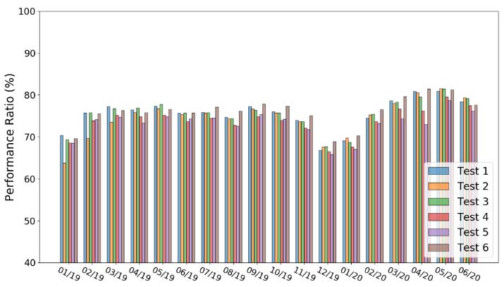
Figure 15. Monthly PR of the six test areas
| Prod 1 | Prod 2 | Test 1 | Test 2 | Test 3 | Test 4 | Test 5 | Test 6 | |
| January 2019 | 65,1 | 71,7 | 70,2 | 63,8 | 69,4 | 68,6 | 68,5 | 69,6 |
| February 2019 | 71,1 | 75,7 | 75,7 | 69,7 | 75,8 | 73,8 | 74,1 | 75,5 |
| March 2019 | 74,3 | 77,9 | 77,2 | 73,5 | 76,7 | 75,2 | 74,6 | 76,3 |
| Q1_2019 average | 70,2 | 75,1 | 74,4 | 69,0 | 73,9 | 72,5 | 72,4 | 73,8 |
| April 2019 | 72,1 | 74,0 | 76,5 | 75,8 | 76,9 | 74,8 | 73,4 | 75,8 |
| May 2019 | 66,9 | 74,6 | 77,3 | 76,7 | 77,8 | 75,2 | 74,8 | 76,5 |
| June 2019 | 70,9 | 75,5 | 75,6 | 75,3 | 75,7 | 73,7 | 74,3 | 75,7 |
| Q2_2019 average | 70,0 | 74,7 | 76,4 | 75,9 | 76,8 | 74,6 | 74,2 | 76,0 |
| July 2019 | 71,0 | 76,0 | 75,9 | 75,7 | 75,7 | 74,4 | 74,5 | 77,1 |
| August 2019 | 69,7 | 74,1 | 74,7 | 74,3 | 74,4 | 72,8 | 72,5 | 76,1 |
| September 2019 | 72,9 | 77,5 | 77,3 | 76,7 | 76,4 | 74,8 | 75,3 | 77,8 |
| Q3_2019 average | 71,2 | 75,9 | 75,9 | 75,6 | 75,5 | 74,0 | 74,1 | 77,0 |
| October 2019 | 73,7 | 78,2 | 76,0 | 75,7 | 75,7 | 73,9 | 74,2 | 77,3 |
| November 2019 | 72,3 | 76,8 | 73,9 | 73,6 | 73,7 | 72,0 | 71,7 | 75,0 |
| December 2019 | 66,8 | 70,9 | 66,8 | 67,6 | 67,6 | 66,5 | 65,8 | 68,9 |
| Q4_2019 average | 70,9 | 75,3 | 72,2 | 72,3 | 72,3 | 70,8 | 70,6 | 73,7 |
| January 2020 | 70,8 | 75,4 | 69,1 | 69,7 | 68,7 | 67,6 | 67,0 | 70,2 |
| February 2020 | 72,3 | 76,8 | 74,5 | 75,2 | 75,4 | 73,7 | 73,2 | 76,5 |
| March 2020 | 74,4 | 79,1 | 78,6 | 78,0 | 78,3 | 76,6 | 74,3 | 79,6 |
| Q1_2020 average | 72,5 | 77,1 | 74,1 | 74,3 | 74,1 | 72,6 | 71,5 | 75,4 |
| April 2020 | 73,0 | 75,6 | 80,8 | 80,6 | 79,5 | 76,2 | 72,9 | 81,4 |
| May 2020 | 75,9 | 81,3 | 80,9 | 81,5 | 81,4 | 79,5 | 78,7 | 81,2 |
| June 2020 | 74,4 | 79,5 | 78,4 | 79,3 | 79,1 | 77,5 | 76,1 | 77,6 |
| Q2_2020 average | 74,4 | 78,8 | 80,1 | 80,5 | 80,0 | 77,5 | 75,9 | 80,1 |
| Total 18 months | 71,5 | 76,2 | 75,5 | 74,6 | 75,4 | 73,7 | 73,1 | 76,0 |
| Average PRtot | 74,5 | |||||||
Table 3. Monthly PR (%) of each zone and average value for the whole period.
Looking at the graphs and at the table, a few observations can be made. In the whole period, production area 2 performed better than production area 1, with an overall PR of around 76% and 71%, respectively. The main cause for this can be attributed to the fact that production area 1 comprises the Moleneind underpass. As shown in Figure 10, in proximity of the underpass four sections (two on each side) overlap, thus casting shade on each other; the PR of those sections are constantly lower than the rest.
Figure 16. Overlapping PV sections in proximity of Moleneind underpass.
During the first year of operation, the test areas have been characterized by PR ranging from around 72% to 76%. Area 6 was usually recording higher PR values thanks to the installation of white concrete tiles on the rear side of the system, meant to enhance the albedo of the surrounding, thus the reflected irradiance and the energy yield (not within the scope of this project). The reason of particularly low performance of some test areas in specific periods (e.g. test area 2 in Q1 2019) were almost entirely due non-optimal functioning of some PV laminates and/or power electronics. After noticing the problems, usually actions were promptly taken to fix and restore the system.
For all areas, December 2019 was the worst month in terms of energy performance. During that month, many days were characterized by extremely low irradiance values, and sometimes parts of the system were momentarily shut down. On the other hand, the best performance was achieved in Q2 2020, specifically during May. The reason why all areas reported a significant increase is the update of the power optimizers’ firmware. After a thorough analysis, it was found that all POs installed in the SH system were underperforming, i.e. not able to find the global maximum power point during construction shading periods. A few of them were fixed starting from January 2020, but most of them started to properly function only after the 30th of April. This is why in May 2020 performance ratios higher than 80% were recorded (the favorable weather also played a role thanks to the sunny but not so hot days). Additional information on the POs issue will be provided in the following sections. All in all, the overall PR of the Solar Highways noise barrier in the complete monitoring period was 74.5%.
3.3. Construction shading
In general, the performance ratio is strongly affected by the construction shading coming from the support structures of the PV elements, which takes place inevitably every day around noon. The time and duration of this shading effect varies depending on the month, as can be seen by the low plateau of the power generation profile curves in Figure 10. To better visualize the impact of construction shading we can look at Figure 17, where the instantaneous power is plotted as function of the effective irradiance.
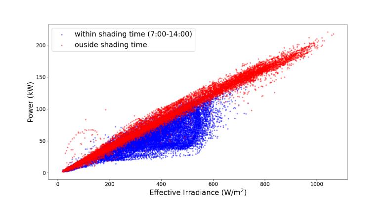
Figure 17. Instantaneous SH power vs. effective irradiance showing the presence of shading.
In the graph, one whole year has been plotted, where power and irradiance measurements are taken every 5-min. Some datapoints follow a linear trend, as expected for any non-shaded PV systems, but many others do not. Taking as shading time-window any minute from 7:00 to 14:00 and assigning the corresponding datapoints a different color (blue), we can see that they clearly lay outside the linear trend, thus proving the presence of shade in that timeframe.
Note that not in every moment of the year the construction shading problem starts occurring at 7 am; in winter months it usually takes place from around 10 am. The quite conservative time-window 7-14 has been chosen to allow to consider all datapoints in the year and to have a better visualization of the problem.
Another way to visualize the problem is by plotting the PR of the overall system as function of irradiance bins, as shown in Figure 18. In the blue columns all data have been considered without filtering for the shading time. It can be observed that in the first three bins the PR has much lower values, especially when the irradiance is between 400 and 600 W/m2. When looking back at Figure 17 we can indeed see that the majority of blue points lays in that irradiance range, therefore when we include them into the calculation, the overall PR decreases. On the other hand, when those values are filtered out, a more expected trend is obtained, as shown by the red columns.
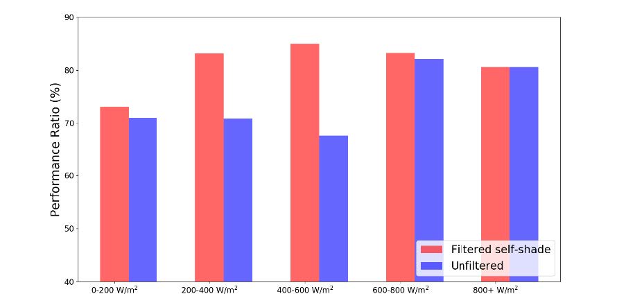
Figure 18. PR as function of irradiance bins for shade-filtered and unfiltered data.
Following the same filtering procedure, e.g. considering only the power production outside the construction shading time, we calculated again the overall yearly PR of the Solar Highways full system. The PR value increases significantly, going from around 73% to 83%. This result underlines the importance of trying to mitigate as much as possible the construction shade caused by the support struction of vertical PV bifacial systems. As it will be explained in the following chapter, the Solar Highways performance was higly affected by this phenomenon, also because of a non-optimal behaviour of the power optimizers.
4. SolarEdge power optimizers investigation
As discussed earlier, due to the nearly-vertical position and the west-east orientation, the solar noise barrier suffers from construction shading caused by its own support structure, which cast a shade on part of the PV modules around noon. To mitigate the negative effect of construction shading, the Solar Highways PV modules have been designed in order to ensure smart placement of the solar cells within the module, smart stringing layout and optimal design of the support structure.
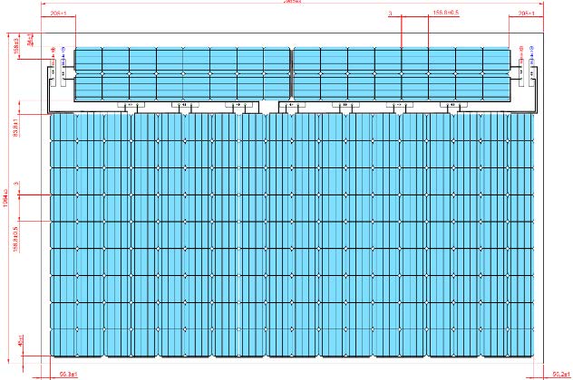
Figure 19. Technical drawing showing the lay-out of the cell placement and stringing of a SH laminate.
Figure 19 shows the cells placement and string layout of the SH PV laminate. The first two row of cells in the top part of the laminate have been grouped with an horizontal stringing, while the rest of the cells have a vertical stringing. All cells are connected in series. In total, 11 bypass diodes are used. Each laminate is connected to two independent power optimizers (POs): the power optimizer on the left side (w.r.t. the figure) deals with 5 substrings of cells (1 horizontal and 4 vertical), while the PO on the right side has 6 substring (1 horizontal and 5 vertical).
The power optimizers used are SolarEdge P800s. These devices are supposed to constantly track the maximum power point of each laminate (or more precisely, “half-laminate”) they are connected to. When they are connected to a SolarEdge inverter, as in our case, they convert each module’s voltage to a fixed voltage for the whole string of modules, hence allowing high flexibility even with long strings and strings with different lengths. Module-level power electronics, as POs, should be able to mitigate shading losses by isolating the impact to the shaded modules, while allowing the rest of the modules in the system to contribute at their full power.
But how do POs handle module-level shading?
In the SH case, all modules of each string connected to an inverter will approximately suffer from the same partial shading condition due to the inevitable construction shade from the support structure. Ideally, each power optimizer should be able to track the maximum power point and force its (half-)module to operate at that point. This means that when some cells become shaded, the bypass diodes of the relative cell-substrings should start conducting. In this way, multiple maximum power points are created and it is duty of the PO to track the global maximum, avoiding the module to operate at one of the local MPPs.
However, by investigating the behavior of the power optimizers from the SolarEdge portal it was found out that almost all POs, for almost all the time, operate the modules at high-voltage local maxima, rather than the global, therefore losing a considerable amount of power. This result has been supported and confirmed by simulations performed with BigEye modelling tool, developed by TNO.
The following graphs show the different behaviors of an optimal and a non-optimal power optimizer on a sunny day, the 21/04/2020. Following the nomenclature used in the SolarEdge web portal, PO 11.1.5 (blue line) represents the non-optimal optimizer, while PO 8.1.6 (orange line) represents the good-performing one.
Figure 20 shows the voltages at module level for the two POs. It can be observed that in the morning, PO 8.1.6 shows a voltage drop of around 15V and another shorter drop in the afternoon right after solar noon. These voltage drops indicate the activation of the bypass diodes. Most likely two bypass diodes are activated, one horizontal and one vertical (horizontal string: 16 cells * 0.55 Vmpp_STC/cell; vertical string: 18 cells * 0.55 Vmpp_STC/cell). When the shaded cells are bypassed, the module current is not anymore limited by them, therefore a higher current can flow. As shown in Figure 21, the morning-peak of the current-curve of PO 8.1.6 is wider than the other one, translating in a narrower plateau around noon. When looking at the power curves in Figure 22, it is possible to see that the well-performing PO produces significantly more power around noon than the non-optimal one. As stated before, the difference in the operation of the two POs is the ability to find and operate the module at the global maximum power point (lower V, higher I), rather than sticking to a local one (higher V, lower I).
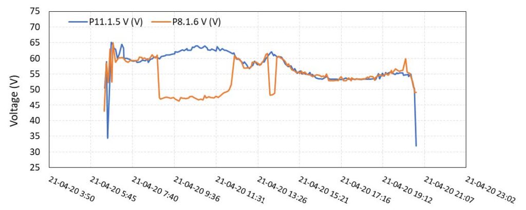
Figure 20. Voltage curves of an optimal and a non-optimal PO during a sunny day (21/04/2020).
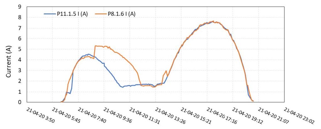
Figure 21. Current curves of an optimal and a non-optimal PO during a sunny day (21/04/2020).
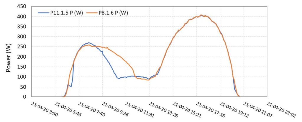
Figure 22. Power curves of an optimal and non-optimal PO during a sunny day (21/04/2020).
The non-optimal behavior of most POs in the Solar Highways noise barrier was pointed out to SolarEdge, which took action and updated the firmware of the devices. Unfortunately, however, not all the POs were fixed on the same day. The whole process took place from January to April 2020. The dates in which the firmware updates were performed are recapped below. To better understand the performance analysis, we included in the list also the dates of some relevant issues/maintenance work done in 2020:
- 15/01/2020 PO firmware update (only few POs start working optimally)
- 19/02/2020 PO firmware update (only 53/268 POs are well-functioning, test areas only have 1 or 2 out of 16 functioning POs)
- 8/04/2020 PO firmware update (test areas 1 and 2 fully functioning 16/16)
- 16/04/2020 PO firmware update (test area 3 fully functioning 16/16)
- 20/04/2020 second round of cleaning
- 30/04/2020 all POs fixed and optimally working (also test area 4 and 5 fully functioning)
- 24/03 to 23/04 one module/PO of area 5 is completely off
To quantify the effect of the POs update on the energy performance of the system, we compare the two power optimizers of the previous example, PO 11.1.5 (in test area 4) and PO 8.1.6 (in test area 1). The PO of test area 1 started to fully function on the 8/04, while the one of test area 4 only on the 30/04. Figure 23 shows the daily energy produced by the two POs and their relative difference.
It can be seen that in the period between 8 and 30 April, the PO of test area 1 produced more energy than the PO in test area 4. The energy difference between the two POs goes from around -3.7% to +3.3%, which means that the POs fixing lead to a yield increase of +7%. After the 30/04, when also the PO of test area 4 is fixed, the difference between the two POs decreases and comes back to negative values. The dips that can be seen in the graph are due to the fact that during cloudy days (especially cloudy mornings), the effect of construction shading is lowered or nulled, so the modules will behave similarly despite the functioning of the POs.
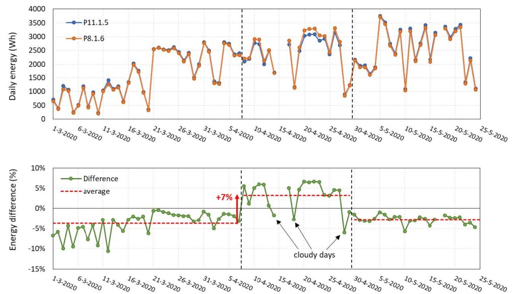
Figure 23. Daily produced energy of one PO of test area 1 (P8.1.6) and one PO of test area 4 (P11.1.5) and relative difference between the two. The dashed black lines indicate the dates of the firmware updates.
The same trend can be observed in Figure 24, where the daily PR of all test areas (except area 6, where the albedo experiment is carried on, thus higher PR values are recorded) are shown for the period going from beginning of February to the beginning of June. The vertical dashed lines indicate the moments of PO updates; within that period we can clearly see the higher performance of T1 and T2 -from the 16/04 onwards also of T3 – compared to the yet-unfixed T4 and T5. The bars represent the absolute difference in PR between the various test areas with respect to T4. The daily PR absolute difference goes on average from +1/2% to + 6/7%, so and absolute PR gain of +5% (corresponding to a +7% relative, in accordance to the value found in the analysis of a single PO on a sunny day).
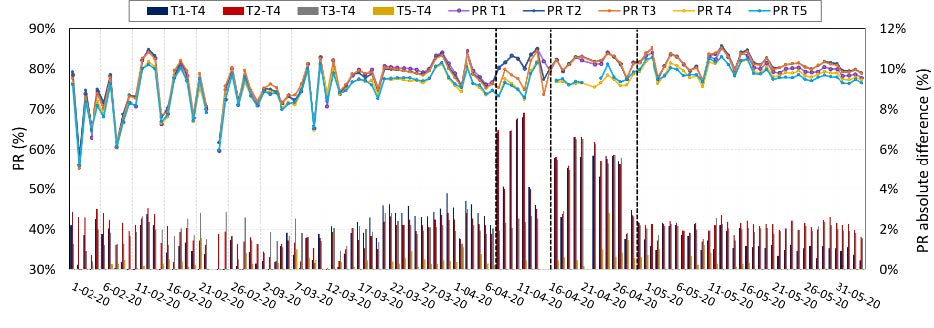
Figure 24. Daily PR and PR (T3-T4) from beginning of February to end of May. The dashed black lines indicate the dates of the firmware updates.
The impact of construction shading for the improved Solar Highways system (equipped with good-working POs) can be seen by looking at Figure 25. The two graphs show respectively the relation between power and effective irradiance in May 2019, when the POs performed sub-optimally, and in May 2020, after they were fixed. The comparison clearly shows that with proper power electronics, the PV modules are able to handle construction shading in a much better way.
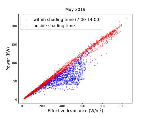
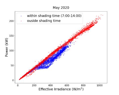
Figure 25. Power vs. effective irradiance in case of non-optimal and optimal behavior of the POs respectively in May 2019 (left) and May 2020 (right).
In conclusion, the analysis revealed the importance of having optimally functioning power optimizers, able to detect the global MMP, especially when the system is subjected to construction shading. The POs firmware update showed an averaged increase in the power production and performance of around +7%. This value gives a clear indication on the importance of this aspect, but it can not be extrapolated to draw conclusions on a yearly possible yield gain/loss. It must be kept into account that the calculations are only based on measured data from May and April 2020, with a typical spring weather that can differ significantly from the summer or winter seasons.
To provide an estimation of this effect on a yearly basics, simulations have been performed with BigEye, the bifacial PV modeling software developed by TNO. At first, the Solar Highways module configuration (i.e. same stringing layout, number of bypass diodes, orientation, etc.) have been reproduced and the model has been validated comparing with the real measurements of April and May 2020. Then, the simulations have been performed for a typical meteorological year, assuming the presence/absence of ideal bypass diodes able to operate the module at the maximum power point. According to the simulations, the inability to find the MPP, hence the non-optimal functioning of the POs, could lead to a power loss of around 3-5%/year.
5. Effect of cleaning
As part of Solar Highways investigation plan, the effect of cleaning on the PV elements’ performance has been evaluated. The 6 experimental areas have been used to test different cleaning regimes, according to the plan shown in Table 4.
| Area | Cleaned side | Frequency | Cleaning dates |
| Test area 1 | Road side (West) | 1 x year | 21-05-2019
20-04-2020 |
| Test area 2 | Resident side (East) | 1 x year | 21-05-2019
20-04-2020 |
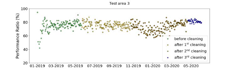
| Test area 3 | Resident side (East) | 2 x year | 21-05-2019 and 24-10-2019
20-04-2020 |
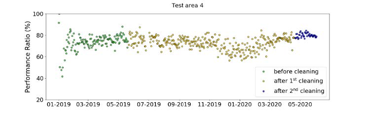
| Test area 4 | No cleaning | ||
| Test area 5 | Both sides | 1 x year | 21-05-2019
20-04-2020 |
| Test area 6 and rest of installation | Both sides | 1 x year | 21-05-2019
20-04-2020 |
Table 4. Cleaning plan
The first cleaning of the PV elements and the aluminum frames took place on the 21st of May 2019. According to the plan, test area 1 was cleaned only on the front west side, area 2 and 3 only on the rear east side, area 4 was not cleaned at all, and area 5 was cleaned on both sides. Area 6, as well as the rest of the solar noise barrier, was also cleaned on both sides. Test area 3 was then cleaned a second time, on the 24th of October 2019, to investigate also the impact of the cleaning frequency. In 2020 the same cleaning schedule was applied, and the cleaning day was 20th of April 2020. The photos in Figure 26 depict two of the cleaning days.
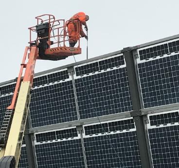
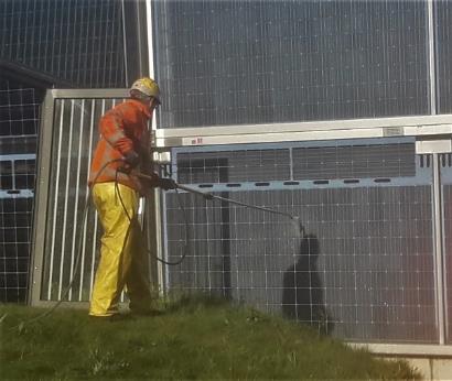
Figure 26. Cleaning of the Solar Highways PV laminates in 2019 (left) and 2020 (right).
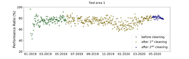
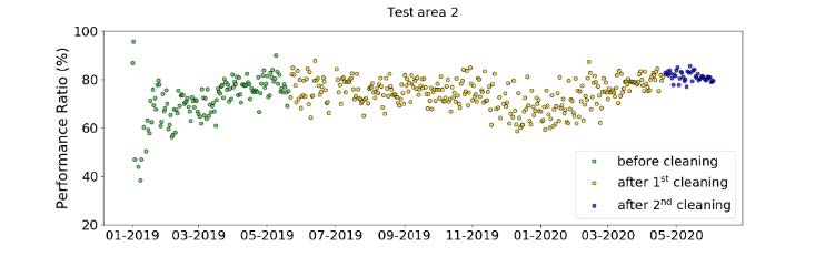
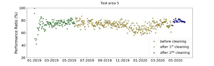
To evaluate the effect of cleaning on the PV performance we looked at the performance ratio of each test area and we compared the PR of the cleaned areas with the PR of the uncleaned one, i.e. test area 4. While the daily PR values (in absolute terms) are shown in Appendix A, the graphs below show the PR difference between each area with respect to area 4. On the y-axis, we will therefore see a relative percentage which indicates the PR gain/loss, or more in general, the difference between two specific areas, for instance
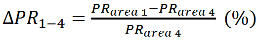
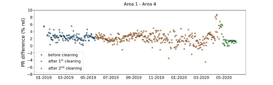
Figure 27. Relative PR difference between test area 1 and 4.
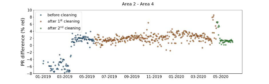
Figure 28. Relative PR difference between test area 2 and 4.
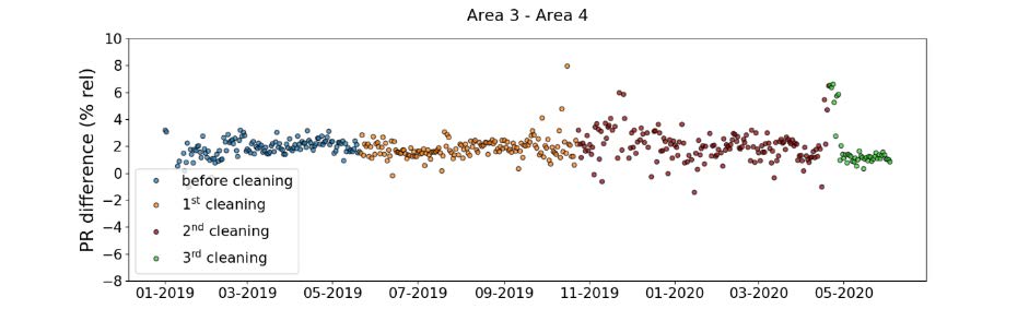
Figure 29. Relative PR difference between test area 3 and 4. Note: first two cleanings in 2019 and third one in 2020.
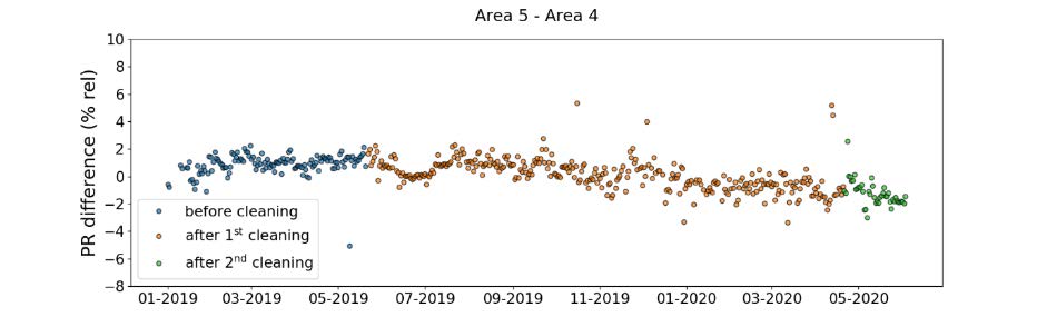
Figure 30. Relative PR difference between test area 5 and 4.
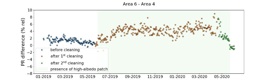
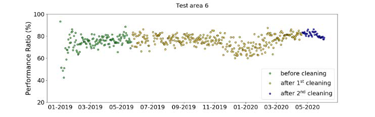
Figure 31. Relative PR difference between test area 6 and 4. Note: the image shows also the presence of the high-albedo patch behind test area 6.
To start, let us focus on the first cleaning (in the plots: the transition from the blue to the orange points). From the graphs, we cannot see a clear PR gain which can be associated to the cleaning. The dots in the graphs show some PR fluctuations, which are dependent on the fact that the different areas might be subjected to slightly different conditions (e.g. on some days there might be shade on one area but not on the other one). The graph of test area 6 should not be considered for cleaning evaluation, since the boost in PR reported there is due to the installation of white concrete tiles with high-albedo on the rear east side of the PV elements, which took place in the same period (29th of May 2019). It is useful, however, to point out the difference between the cleaning and the albedo experiments: while the increased albedo of the surrounding area had a clear positive impact on the performance, the cleaning of the modules did not show a significant effect.
Evaluating the effect of the second cleaning round, performed in April 2020, is even less straightforward compared to the first time. This is because in the same time period many issues overlapped: cleaning, updating of the power optimizer firmware, malfunctioning of a full laminate of test area 5, short shut-downs due to maintenance work. In particular, as discussed in the previous chapter, fixing the firmware of the POs resulted to have a strong positive impact on the performance. The fact that the fixing process did not happened in one go but took place gradually from January to April 2020 makes more difficult to distinguish between the various issues. The relevant dates in which the POs firmware were updated are summarized in the timeline shown below, which states also the exact number of POs that started to function properly for each test area. The overview is essential to be able to decouple the effect of POs’ fixing and the effect of cleaning.
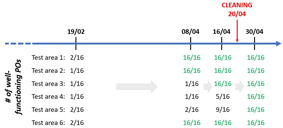
Figure 32. Timeline showing actual number of functioning POs for each test area after the dates of POs firmware’s update.
As can be seen, test areas 1, 2 and 6 were fully functioning already since the 8th of April, while for test area 3, 4 and 5 the fixing process was more gradual; only on the 30th of April all test areas were properly fixed. The effect of the POs fixing is significant and makes the evaluation of the cleaning process, which happens in the same period and it is expected to be small, rather difficult. Figure 33 zooms in on the PR difference between the single test areas when compared to area 4 (the uncleaned one), similarly to the graphs shown before. The gaps are due to missing data in occurrence of maintenance work. The increase that we see in some curves is not due to cleaning, but to the POs update. The behavior of the single curves can be understood when looking at the timeline with the POs fixing. The curves of (T1-T4) and (T2-T4) go up after the 8th of April (when all their POs are fixed, while T4’s POs are still malfunctioning); (T3 – T4) on the other hand remains constant since the POs of both area 3 and 4 are not yet fixed. On the 16th, T4 has around a quarter of its POs well-functioning, so the curves go slightly down; finally, around the 30th when also T4 has all its POs fixed, all the curves go back to values of around +2/3%, as they were before the 8th of April, i.e. before the cleaning. T5 shows a decreased performance because one of its laminate was not working at all from 24/03/2020 to 23/04/2020. When the problem was solved we see an increase in its PR.
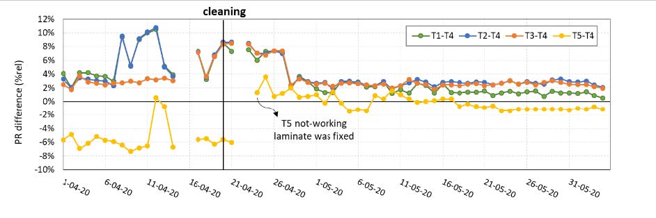
Figure 33. PR difference between cleaned (T1, T2, T3, T5) and uncleaned (T4) test areas in the period of the second cleaning. The graph mostly shows the effect of the POs firmware update.
The performance ratio and power curves for single days before and after the cleaning days have also been analyzed, in order to see a possible instantaneous power increase during mornings or afternoons. Test areas 2 and 3, cleaned on the rear east side, were expected to show an increased PR during morning hours, while area 1, cleaned on the front west side, an increase during the afternoon. Area 5 was expected to perform better over the whole day, since cleaned on both sides. However, none of the cases showed the expected behavior. As an example, Figure 34 shows power and PR of test area 1 and 4 for a sunny day before (top graphs) and after (bottom graphs) the cleaning. Area 1 was cleaned on the west side, but we cannot see any increase in performance in the afternoon hours. Area 1 was already performing better (+2/3%) than area 4, even before the cleaning.
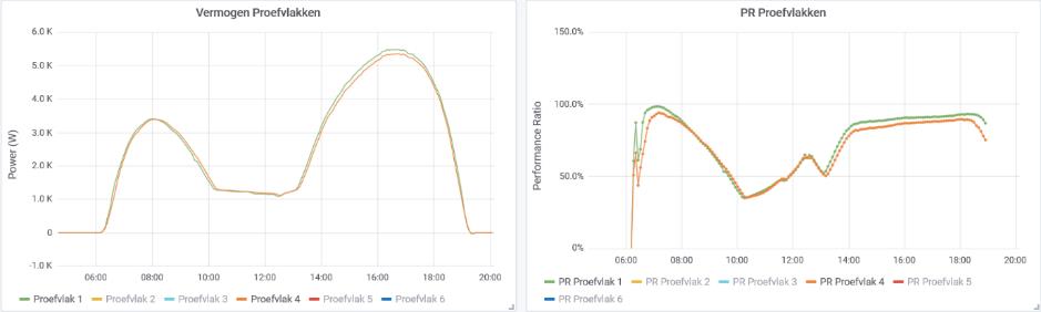
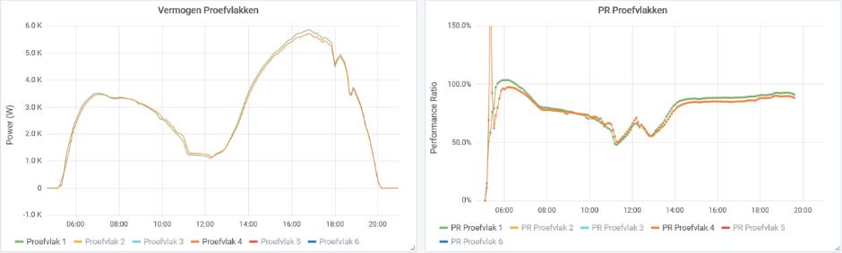
Figure 34. Power and PR curves (T1 and T4) on a sunny day before (5/04/2020, top graphs) and after (6/05/2020, bottom graphs) the second cleaning.
As observed after the first cleaning in 2019, also the second round did not show any significant improvement in the energy performance of the Solar Highways. Given the large size of the system, the customized panels, and all the practical issues mentioned before, the results of the cleaning evaluation cannot be provided with a further degree of accuracy. In this case, increasing the accuracy of the results would risk to be meaningless and misleading, since the same accuracy is not met in the monitoring conditions. However, it can be concluded that the PV modules of the Solar Highways are not heavily affected by soiling and particles accumulation. The almost-vertical tilt of the structure likely helps in avoiding dust accumulation and facilitate the self-cleaning due to rainfall. To conclude, due to the absence of a significant positive effect, cleaning procedures are not considered necessary for the Solar Highways noise barrier for the purpose of increased energy output.
6. Vandalism
During the monitoring phase, a number of acts of vandalism were encountered. Despite damage, no lasting effect of decreased power output was observed.
6.1. Graffiti
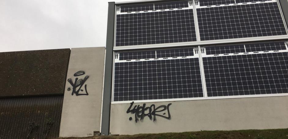
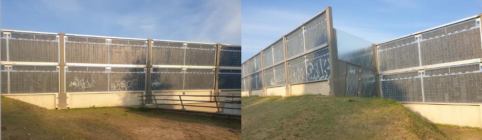
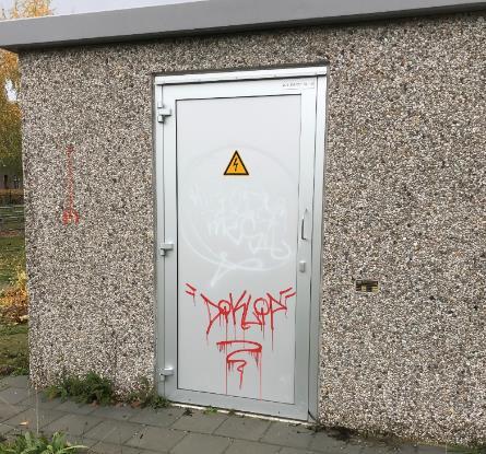
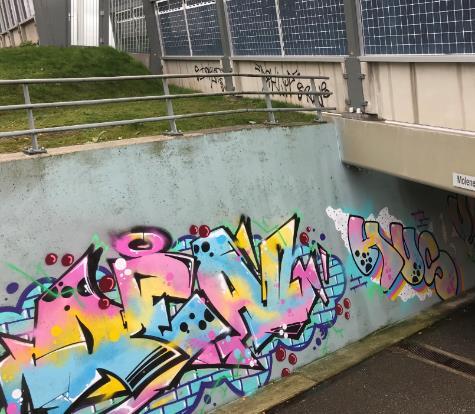
Figure 35. Examples of graffiti found on the PVNB and on the surroundings.
Graffiti were encountered a number of times. At first only graffiti were found on the parts of the system that does not produce power, e.g. the concrete parts. Later, also parts of the PV-active surface were covered. Figure 35 shows examples of graffiti found on the noise barrier and the surroundings. The municipality had suspicions about the person(s) involved and explained to them that also the rear side generates renewable energy. After that, no graffiti were found on the photo-active areas. The affected areas were cleaned.
6.2. Other vandalism
Other acts of vandalism were encountered. In a number of cases, the glass on one side of a number of laminates broke. Most likely these damages were caused by rock-throwing. Clear marks of impact were seen. Figure 36 shows examples of these breakages. In two cases the cassettes were replaced.
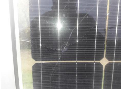
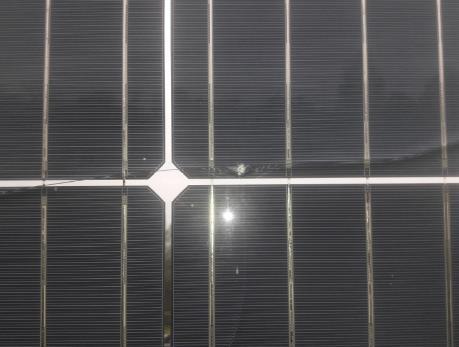
Figure 36. Damages to the Solar Highways noise barrier PV laminates.
Damage to one of the cabinets containing the grid connection and electronics was encountered, where the hinges and the door were damaged. Also, the effect of fireworks is visible (Figure 37, left). This was first temporarily repaired (Figure 37, right), later more permanently.
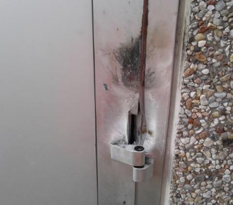
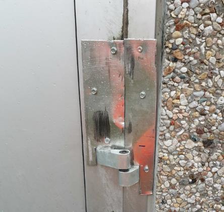
Figure 37. Damages to the Solar Highways electronics cabin.
7. Verifying Techno-Financial Model
In 2015, SEAC wrote the report ‘Solar Highways, wat levert het op?’², which describes business cases for operating a solar noise barrier. This report was written before the procurement procedure of the Solar Highways noise barrier was started, and therefore based on a number of assumptions for cost price. For the value of the electricity, it makes a large difference how the electricity is sold. The least beneficial scenario was a net-metering scenario, where the income from the electricity produces is equal to the avoided cost for the electricity bought from the grid. In this case the value of a kWh is estimated at €0.04/kWh. The most beneficial scenario is a scenario where the energy is sold through an energy cooperation, making use of the Regeling Verlaagd Tarief (RVT) or Postcoderoos, where members are exempted from paying energy tax.
In this section, we will investigate how the real CAPEX, OPEX and the value of electricity compare to the assumptions from the report. Furthermore we will calculate the consequences for the business case of the Solar Highways noise barrier.
²Minne de Jong, Solar Highways: Wat levert het op?, Een techno-financiële uitwerking van verschillende inkomstenscenario’s voor het Solar Highways project, nu en in 2020, SEAC, November 2015
7.1. CAPEX
In our original model, we calculated the ‘added’ cost per kWh and m2 of a bifacial noise barrier compared to a standard noise barrier. In the ‘2015’ scenario, we estimated this added cost to be €256/m2 or €2/Wp. The €2/Wp was built up as follows:
- PV module (cassette) cost: €2.22/Wp
- Balance of System (BOS) cost: €0.63/Wp
- Avoided cost (no cost for glass cassettes) : €0.85/Wp
- Total added cost: €2.00/Wp
After the procurement procedure, the cost per m2 turned out to be significantly higher than anticipated. As a complete breakdown in components cost is not available, we present our best estimation. A breakdown into PV module and BOS is needed as input for the model. The estimated Solar Highways cost breakdown is as follows:
- PV module (cassette) cost: €4.42/Wp
- Balance of System cost: €0.63/Wp
- Of which €0.23/Wp for power electronics (inverters etc)
- Of which €0.40/Wp other BOS
- Avoided cost (no cost for glass cassettes) : €0.86/Wp
- Total added cost: €4.19/Wp (or 649 €/m2 or 1.04 M€ total )
7.2. OPEX
The cost for operation and maintenance can have a large influence on the business case. Cleaning of the system could be one of the main cost drivers here. After 18 months of monitoring, we did not find a measurable positive influence of cleaning the modules, as described in the chapter ‘Effect of cleaning’. Therefore we do not anticipate costs for cleaning. In the early phase after commissioning there were a number of issues. We will not take these as OPEX, but as being part of the commissioning of the system. Furthermore, repair works were needed as a consequence of acts of vandalism.
Based on estimations from Rijkwaterstaat, the yearly costs for OPEX is estimated at €20,500, or €0.083/Wp. Without taking into account inverter replacement this amounts to €18,000, or 1.8% of the investment cost (without inverters). In our report we estimated a yearly O&M cost of 1.5% of the initial investment cost. These numbers include safety checks, monitoring software, network connection fees, saving up for inverter replacements (incl work) and damage repairs. 20% was added for unforeseen costs. Roughly half of this number is reserved for damage repairs.
7.3. Value of electricity
In the Solar Highways project citizens living near the noise barrier were involved in the project. A local energy corporation was engaged to set a RVT (or Postcoderoos) project. To date, this was not successful, mainly due to legal issues. Therefore, now the produced electricity is net-metered by Rijkswaterstaat, with as a consequence, a relative low value for the electricity. We estimate the value at €0.04/kWh. I f we take into account the yearly projected production of 203 MWh, this leads to a total value of 8 k€ of the electricity. With the use of the RVT the value of electricity increases to €0.154/kWh or 31k€. This is not the same as the income for Rijkswaterstaat, when Rijkswaterstaat chooses to ground lease the installation to an energy cooperation, as such a cooperation will have costs for organization, administration and take an operational risk by leasing the installation. The value of a ground lease contract is estimated between 18 and 19 k€ by Rijkswaterstaat.
Although Rijkswaterstaat wished to involve local inhabitants, they also formulated that a return of taxes (such as for the RVT), does not decrease the cost for the state as a whole, but does increase the administrative load. Therefore using the RVT may increase the value of electricity for this project, it does not benefit the financial situation of the state as a whole and may therefore not be the optimal situation.
7.4. The Solar Highways business case
When we use these numbers for the business case for Solar Highways, we find that in all scenarios the market value of the produced electricity cannot account for the O&M costs, resulting in a negative Return in Investment and negative Net Present Value.
7.5. Discussion
The CAPEX for the Solar Highways solar noise barrier was much higher than foreseen. The main reason for this is the unique nature of the system. All modules were made by hand in the Netherlands, resulting in a much higher cost price than normal solar modules. If the modules can be made in a high volumes highly automated process, costs will go down. Furthermore, a relatively expensive power electronics system was used. Because the atypical power output of the modules, only largely oversized power electronics were available. Also the six experimental areas, each with a separate inverter increased the price of the system.
Regular large roof-mounted or land-based systems are built and operated by companies that are highly specialized in efficiently designing, preparing and building solar installations. This experimental pilot was built with different goals in mind and built, designed and operated by differently operating entities.
With cost reductions for the components and efficiency improvements in the tendering and building process, costs may be able to go down to a level that will result in a positive net present value and return on investment.
8. Conclusions
Solar Highways, currently holding the record of the world’s largest bifacial solar noise barrier, resulted to be a successful example of PV integration in infrastructure. To answer to the many practical questions related to the actual performance and maintenance of such a system, the noise barrier was monitored since commissioning for a period of 18 months, going from the 1/01/2019 to 30/06/2020.
The net yearly energy yield for 2019 was found to be 202.8 MWh/year, corresponding to an AC specific yield of 816.8 kWh/kWp. This amount of clean electricity could be used to power around 60 typical Dutch households. The total energy output of the 18-month period amounts to 325,5 MWh, with an overall performance ratio of 74.5%.
Thanks to the vertical east-west orientation of the bifacial PV panels, the SH system was able to capture light and generate electricity since the early hours of the morning to the late hours of afternoon-evening. During a typical sunny day, the power profile follows indeed a double-peak shape with a dip around solar noon, when only diffuse light reaches the two sides of the solar modules. The monitoring results also showed the impact of construction shading on the SH performance, i.e. the shading generated by the support structures of the PV laminates, which occurs inevitably every day around noon. To mitigate this problem the Solar Highways modules have been optimally designed in terms of both solar cells placements within the module and cells stringing layout, and they have been equipped with module-level power optimizers. However, it was found that for more than one year the POs were not-optimally functioning due to their inability to find and operate the modules at the global maximum power point in partial shading conditions. The problem was solved thanks to a firmware update from the manufacturer; after fixing the POs, yield and performance increased around 7%. With simulations, it was estimated that in 2019 the system suffered a loss of 3% to 5% because of this problem. This investigation revealed that for vertical bifacial PV systems it is of extreme importance to have not only an optimal module’s design, but also proper power electronics able to handle construction shading.
Furthermore, we investigated the effect of soiling and dust accumulation on the SH modules and the impact of cleaning. For the business case of such a PV- infrastructure integrated system, information on cleaning is crucial to assess the O&M cost. For the investigation, 5 different test areas were cleaned with different cleaning schedules, e.g. by varying frequency and/or the side that was cleaned. One test area was left uncleaned for the whole period, to be able to compare to an uncleaned situation. It was found that none of the cleaning events showed a measurable positive effect on the performance of the PV system. Therefore, it can be concluded the SH is not heavily affected by soiling and particles accumulation, most likely because of the almost-vertical tilt of the structure which may facilitate the self-cleaning due to rainfall. Based on these findings, cleaning procedures are not considered necessary for the Solar Highways noise barrier for the purpose of increased energy output.
During the monitoring period, a few events of vandalism occurred, such as graffiti and module damages probably caused by rock throwing. However, actions were promptly taken to restore the system and no impact on the yield was found.
The CAPEX for the Solar Highways solar noise barrier was much higher than foreseen. In all income scenarios this leads to higher O&M costs than income generated by using or selling the electricity. This leads to a negative Return in Investment and negative Net Present Value.
With cost reductions for the components and efficiency improvements in the tendering and building process, costs may be able to go down to a level that will result in a positive net present value and return on investment.
Appendix A: Daily PR of test areas before and after cleanings